Introduction: Why This Formula Matters
In Microsoft Excel, most people still waste time manually searching data.
But the excel filter function formula changes everything.
Instead of scrolling and selecting manually, you type one formula—and Excel shows only what you need.
This guide will teach you one step at a time, so you never feel confused.
Step 1: Understand Your Data First
Before using FILTER, you must know your data structure.
Example Table:
| A (Name) | B (Class) | C (Marks) |
|---|---|---|
| Ali | 10 | 85 |
| Sara | 10 | 92 |
| John | 9 | 78 |
📸 Step 1 Visual (Look at your data)


6
👉 Just understand:
- Column A = Names
- Column B = Class
- Column C = Marks
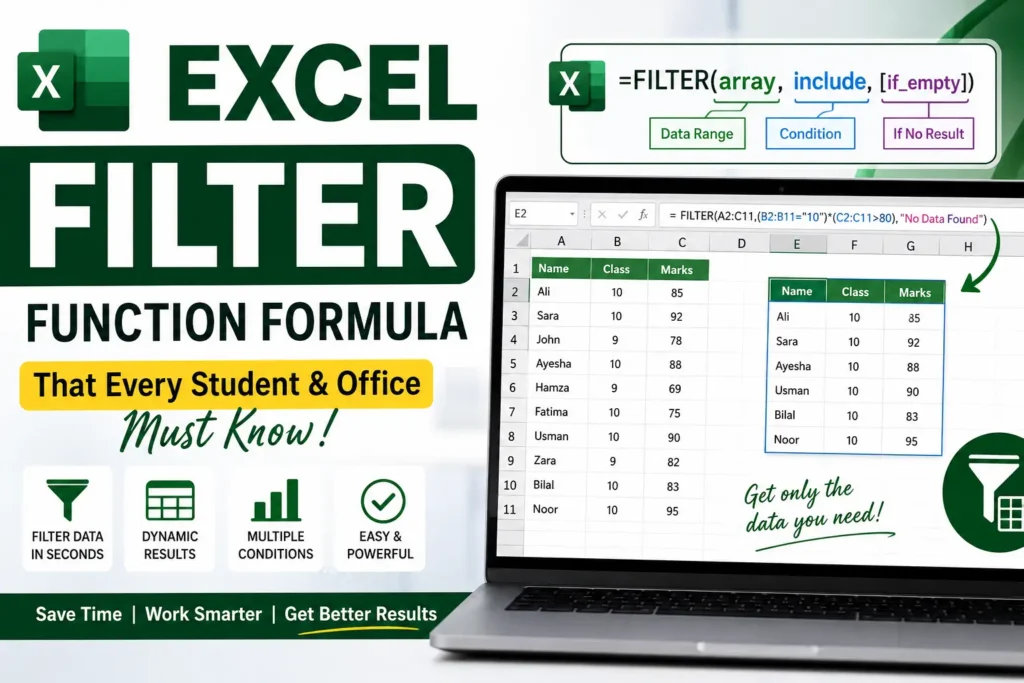
Step 2: Basic FILTER Formula Structure
Now learn the formula slowly.
Formula:
=FILTER(array, include)Meaning in simple words:
- array → whole data
- include → condition
📸 Step 2 Visual (Formula bar explanation)


6
👉 Don’t worry about complexity—just remember:
“Data + Condition = Result”
Step 3: First Simple Example (Very Important)
Now we apply it.
Goal:
Show only Class 10 students.
Formula:
=FILTER(A2:C4, B2:B4=10)What happens?
Excel:
- checks Class column
- finds “10”
- shows only those rows
📸 Step 3 Visual (Output result)


6
Step 4: Understanding “Spill” Result
When FILTER works, Excel automatically expands results.
This is called dynamic array spill.
👉 You don’t drag anything
👉 You don’t copy anything
👉 Excel fills cells automatically
📸 Step 4 Visual (Spill effect)


6
Step 5: Add One Condition (Easy Level)
Goal:
Class 10 students only
Formula:
=FILTER(A2:C10, B2:B10=10)👉 This is called single condition filtering
📸 Step 5 Visual


5
Step 6: Add Two Conditions (AND Logic)
Now slightly advanced—but still simple.
Goal:
Class 10 + Marks above 80
Formula:
=FILTER(A2:C10, (B2:B10=10)*(C2:C10>80))Simple meaning:
*= AND- Both conditions must be true
📸 Step 6 Visual


7
Step 7: Add OR Condition (Very Useful)
Goal:
Class 9 OR Class 10 students
Formula:
=FILTER(A2:C10, (B2:B10=9)+(B2:B10=10))Simple meaning:
+= OR- Any condition can be true
📸 Step 7 Visual


8
Step 8: Handle Empty Results (Important)
Sometimes no data matches.
Instead of error, show message.
Formula:
=FILTER(A2:C10, B2:B10=11, "No Data Found")👉 This makes your report professional.
📸 Step 8 Visual


6
Step 9: Real Office Example (Very Important)
Scenario:
Sales data in office
| Rep | Region | Sales |
|---|---|---|
| Ali | North | 5000 |
| Sara | South | 7000 |
Goal:
North region sales above 5500
Formula:
=FILTER(A2:C10, (B2:B10="North")*(C2:C10>5500))📸 Step 9 Visual


6
Final Understanding (Very Simple)
The excel filter function formula is just:
“Tell Excel what you want → it gives exact results instantly”
No manual work
No confusion
No extra steps