Introduction
If you still use VLOOKUP in Excel, you are probably spending more time fixing formulas than actually analyzing data. That is exactly why the XLOOKUP Formula in Excel became one of the most important Excel upgrades in recent years.
I still remember the first time I used XLOOKUP while managing a student marks sheet. One wrong column number in VLOOKUP broke the entire sheet. After switching to XLOOKUP, the process became faster, cleaner, and much easier to understand.
Whether you are a student, office worker, freelancer, or beginner learning Excel, XLOOKUP can save hours of manual work. It helps you search for values quickly, return matching information, and reduce formula errors.
In this guide, you will learn:
- What XLOOKUP is
- Why it is better than VLOOKUP
- XLOOKUP Formula syntax
- Beginner-friendly examples
- Real-world practical uses
- Common mistakes to avoid
- Advanced tips in simple language
What is XLOOKUP in Excel?
The XLOOKUP Formula in Excel is a modern lookup function used to search for data in a table or range.
It can:
- Search vertically or horizontally
- Return exact matches by default
- Search from left to right or right to left
- Replace both VLOOKUP and HLOOKUP
- Handle missing values more cleanly
Microsoft introduced XLOOKUP to make lookup formulas easier and more powerful.
You can learn more from the official Microsoft Excel Support documentation.
Image: Understanding XLOOKUP Basics


6
Why Beginners Love XLOOKUP
Here is why most Excel users now prefer XLOOKUP:
| Feature | VLOOKUP | XLOOKUP |
|---|---|---|
| Searches left to right | Yes | Yes |
| Searches right to left | No | Yes |
| Exact match default | No | Yes |
| Easier syntax | Medium | Easy |
| Column number required | Yes | No |
| Error handling | Difficult | Simple |
The biggest advantage is simplicity. You no longer need to count columns manually.
XLOOKUP Formula Syntax
Here is the basic syntax:
XLOOKUP(lookup_value,lookup_array,return_array,[if_not_found],[match_mode],[search_mode])
Explanation of Each Argument
| Argument | Meaning |
|---|---|
| lookup_value | The value you want to search |
| lookup_array | The column or row containing the value |
| return_array | The data you want returned |
| if_not_found | Optional message if no match exists |
| match_mode | Controls exact or approximate matching |
| search_mode | Controls search direction |
At first, the formula may look long, but in practice it is easier than VLOOKUP.
Simple Student Marks Example
Imagine you have this Excel table:
| Student Name | English | Math | Science |
|---|---|---|---|
| Ali | 78 | 85 | 80 |
| Sara | 90 | 88 | 91 |
| Ahmed | 67 | 72 | 70 |
Now you want Excel to return Sara’s Math marks automatically.
Use this formula:
=XLOOKUP(“Sara”,A2:A4,C2:C4)
Result:
88
This formula tells Excel:
- Search for “Sara”
- Look inside cells A2:A4
- Return the matching value from C2:C4
That is it.
Image: Student Marks XLOOKUP Example


6
Step-by-Step Guide to Use XLOOKUP
Step 1: Prepare Your Data
Organize data in columns properly.
Example:
| ID | Employee Name | Salary |
|---|---|---|
| 101 | Hamza | 50000 |
| 102 | Bilal | 65000 |
| 103 | Ayesha | 72000 |
Clean data makes formulas more accurate.
Step 2: Select the Result Cell
Click the cell where you want the result to appear.
Example: E2
Step 3: Enter the Formula
=XLOOKUP(102,A2:A4,C2:C4)
Excel searches for ID 102 and returns the salary.
Result:
65000
Step 4: Press Enter
Excel instantly displays the matching value.
That is the beauty of XLOOKUP.
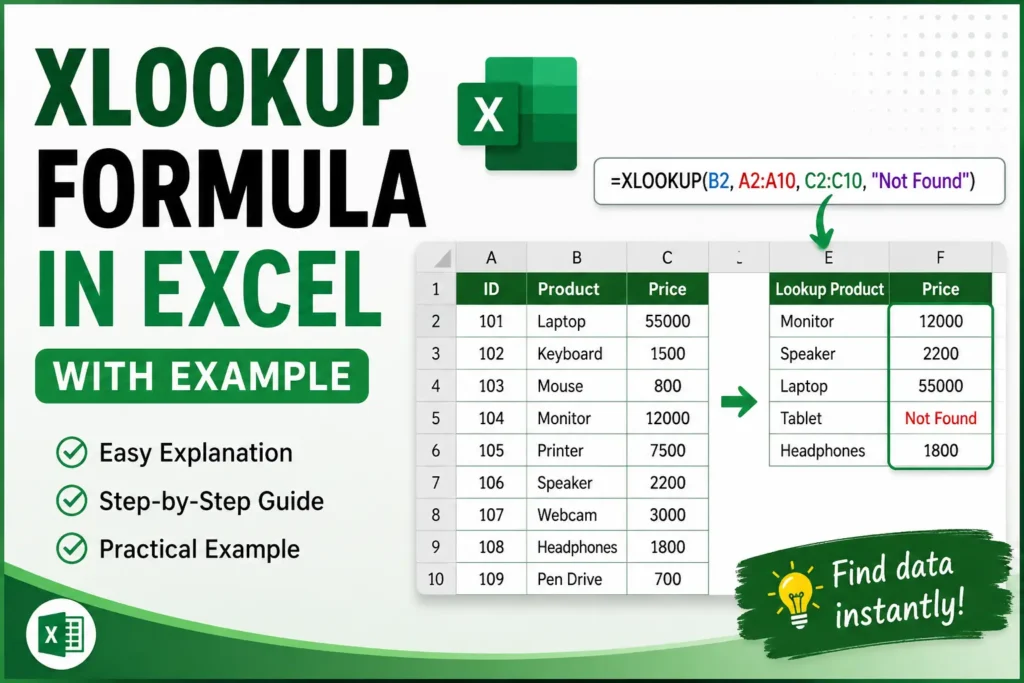
Using XLOOKUP with “Not Found” Message
One of the most useful features is custom error handling.
Instead of showing ugly errors like:
#N/A
You can display a friendly message.
Example:
=XLOOKUP(“Usman”,A2:A4,B2:B4,”StudentNotFound”)
If Usman does not exist in the table, Excel will display:
Student Not Found
This looks far more professional in reports.
Image: XLOOKUP Error Handling


6
XLOOKUP vs VLOOKUP
Most beginners ask:
“Should I learn VLOOKUP first?”
The short answer is: learn XLOOKUP first if your Excel version supports it.
Why XLOOKUP is Better
1. No Column Number Counting
VLOOKUP requires column index numbers.
Example:
=VLOOKUP(A2,B2:E10,3,FALSE)XLOOKUP is cleaner:
=XLOOKUP(A2,B2:B10,D2:D10)2. Searches in Any Direction
VLOOKUP only searches left to right.
XLOOKUP can search both directions.
3. Exact Match by Default
VLOOKUP can produce wrong results if FALSE is forgotten.
XLOOKUP avoids this issue.
4. Easier Maintenance
If columns move, XLOOKUP formulas usually continue working.
That saves a lot of frustration.
Real-World Uses of XLOOKUP
The XLOOKUP Formula in Excel is not just for students. Businesses use it daily.
Office Work
- Employee records
- Salary lookups
- Attendance sheets
Sales & Inventory
- Product prices
- Stock management
- Invoice automation
Education
- Student marksheets
- Attendance tracking
- Grade calculation
Freelancing
- Client databases
- Payment tracking
- Reporting dashboards
Image: Real-World XLOOKUP Uses


6
Advanced Beginner Tips
Use Named Ranges
Instead of:
A2:A100Use named ranges like:
EmployeeIDsThis makes formulas easier to read.
Combine with IFERROR
Although XLOOKUP already handles errors well, combining formulas can create cleaner spreadsheets.
Use Dynamic Tables
Excel Tables automatically expand when new data is added.
This keeps XLOOKUP formulas flexible.
Common XLOOKUP Mistakes
1. Different Range Sizes
Wrong:
=XLOOKUP(A2,B2:B10,C2:C5)The arrays are different sizes.
Always keep ranges equal.
2. Extra Spaces in Data
Sometimes “Ali ” and “Ali” look identical but are different because of spaces.
Use:
TRIM()to clean data.
3. Using Older Excel Versions
XLOOKUP works in:
- Excel 365
- Excel 2021
- Modern Excel Online versions
Older versions may not support it.
You can check compatibility on Microsoft Office Official Website.
Practical Mini Project for Beginners
Try building this simple project:
Student Result Finder
Create columns:
| Roll No | Name | Total Marks |
|---|---|---|
| 1 | Ali | 450 |
| 2 | Sara | 480 |
| 3 | Ahmed | 390 |
Now create a search box.
When you type a student name, XLOOKUP automatically returns marks.
Formula:
=XLOOKUP(F2,B2:B4,C2:C4,”NoRecord”)
This small project teaches real-world Excel automation.
Image: Beginner Excel Mini Project


4
Best Practices for Using XLOOKUP
Keep Data Organized
Messy spreadsheets create formula errors.
Use Tables Instead of Random Ranges
Tables improve readability and automation.
Test with Small Data First
Practice with 5–10 rows before large datasets.
Learn Keyboard Shortcuts
Excel becomes much faster when combined with shortcuts.
Useful resource:
Final Thoughts
The XLOOKUP Formula in Excel is one of the easiest ways to make your spreadsheets smarter and more professional.
For beginners, it removes many frustrations caused by older lookup formulas. Instead of memorizing complicated syntax, you can focus on solving real problems faster.
Once you understand XLOOKUP, you will notice a huge improvement in:
- Speed
- Accuracy
- Spreadsheet organization
- Confidence using Excel
Start with simple examples, practice daily, and gradually use XLOOKUP in real projects like marksheets, employee records, or inventory tracking.
That is how Excel skills grow naturally.
Conclusion
Learning the XLOOKUP Formula in Excel is one of the smartest decisions for anyone working with spreadsheets. It simplifies data searching, reduces errors, and makes Excel far more powerful for everyday tasks.
The best part is that you do not need advanced Excel knowledge to start using it. Even beginners can create professional spreadsheets within minutes.
Now it is your turn.
Open Excel, create a small table, and practice the examples from this guide. The more you experiment, the faster you will master XLOOKUP.
If you found this guide helpful, share it with friends or coworkers who are learning Excel, and explore more beginner Excel tutorials to continue improving your skills.